What is exploratory data analysis| Data Preparation Guide 2024

Market analysis with exploratory data analysis

Now perform exploratory data analysis on market analysis data. You start by importing all necessary modules.

Figure 3: Importing necessary modules

Then you read the data in as a pandas dataframe.

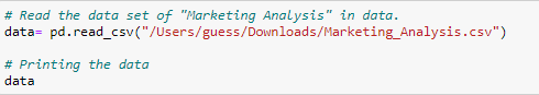
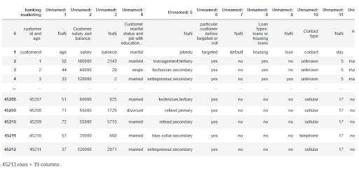
Figure 4: Market Analysis Data

The dataset is not formatted correctly. The first two rows contain the actual column names, just arbitrary values.

Entering data

When entering your data, skip the first two rows to overcome the skewed rows. This will ensure that your column names are filled in correctly.

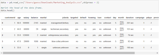
Figure 5: Importing market analysis data

The dataset is now imported correctly. The column names are in the correct order, and you have dropped the arbitrary data.

The above data was collected while taking a survey. Information about the surveys, such as their occupation, salary, whether they have taken a loan, age, etc., is given. You will use exploratory data analysis to find patterns in this data and correlations between columns. You will also perform basic data cleansing steps.

Data cleaning

The next step is cleaning data. Let’s leave the customer ID column because it’s just the row numbers indexed at 1. Also divide the ‘jobedu’ column into two: one for the job and one for the education field. After splitting the columns, you can drop the ‘jobedu’ column as it is more useless.

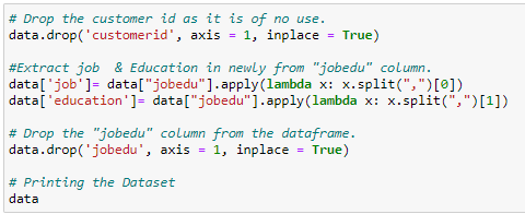
Figure 6: Cleaning market analysis data

This is what the dataset looks like now.

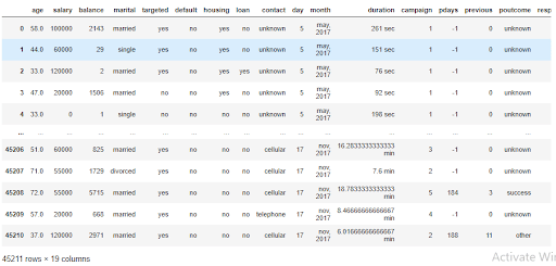
Figure 7: Market Analysis Data

Missing values

The data has some missing values ​​in its columns. There are three main categories of missing values:

MCAR (Missing Completely at Random): These values ​​are missing at random and do not depend on any other values. MAR (Missing Random): These values ​​depend on additional features. MNAR (Not Missing at Random): There is a reason why these values ​​are missing.

Let’s look at the columns that have missing values.

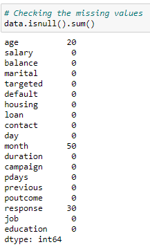
Figure 8: Missing values

You cannot do anything about the missing age values. So leave all rows without age values.

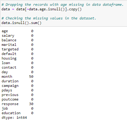
Figure 9: Missing age values

Now, in the month column, you can fill in the missing values ​​by finding the most common month and filling it in place of the missing values. You view the mode of the month column to get the most common values ​​and fill in the missing values ​​using the fill function.

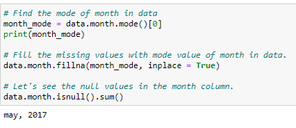
Figure 10: Fill in missing monthly values

Check to see the number of missing values ​​in your data.

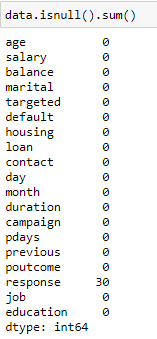
Figure 11: Missing values

Finally, only the answer column has missing values. You cannot change these values. If the user didn’t fill in the answer, you can’t auto-generate it, so you omit these values.

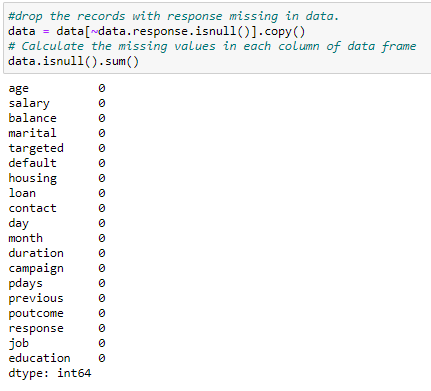
Figure 12: Drop Missing response values

Finally, the data is clean. You can now start to find the outliers.

Handling of outliers

There are two types of outliers in data:

Univariate outliers: Univariate outliers are the data points whose values ​​lie outside the expected range. Here only a single variable is considered. Multivariate outliers: These outliers depend on the correlation between two variables. While plotting data, one variable may not lie outside the expected range. However, when you plot the same variable with another variable, these values ​​may lie far from the expected value.

Univariate analysis

Now consider the different jobs you have data on. Plotting the job column as a bar graph in ascending order of the number of people working in that job tells us the most popular jobs in the market. Normalize the data to ensure they lie in the same range and are comparable.

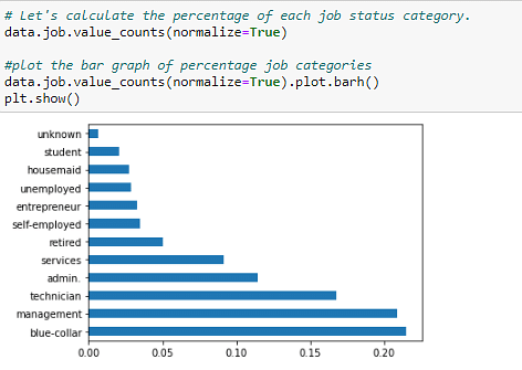
Figure 13: Draw the number of people performing a certain job

Continuing, draw a pie chart to compare the educational qualifications of the people in the survey. Almost half of the people have only secondary school education, and one fourth have a tertiary education.

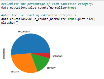
Figure 14: The plot of the educational qualification of people

Bivariate analysis

Bivariate analysis is of three main types:

1. Numerical-Numerical Analysis

When both variables are compared, they have numerical data, and the analysis is said to be a Numerical-Numerical Analysis. You can use scatter plots, pair plots, and correlation matrices to compare two numeric columns.

Scatter plot

A scatter plot represents each data point in the graph. It shows how the data in one column fluctuates according to the corresponding data points in another column. For example, set a scatter diagram between different individuals’ salaries and bank balances and the balance and age of individuals.

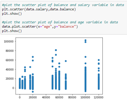
Figure 15: Draw a scatter diagram of Salary vs. Balance

Looking at the above plot, it can be said that regardless of the individual salary, the average bank balance ranges from 0 – 25.0000. Majority of the people have a bank balance below 40k.

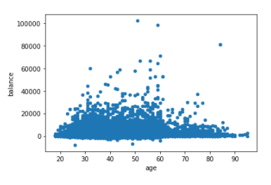
Figure 16: Draw a scatter plot of Balance vs Age

From the above graph you can deduce that the average balance of people, regardless of age, is around 25,000. This is the average balance regardless of age and salary.

Couple Plot

Pair plots are used to compare several variables simultaneously. They plot a scatter diagram of all input variables against each other, which helps save space and allows us to compare multiple variables at once. Let’s draw the pair plot for salary, balance and age.

Figure 17: The plot of a pair plot

The figures below show the pair plots for salary, balance and age. Each variable is plotted against the other on both the x- and y-axis.

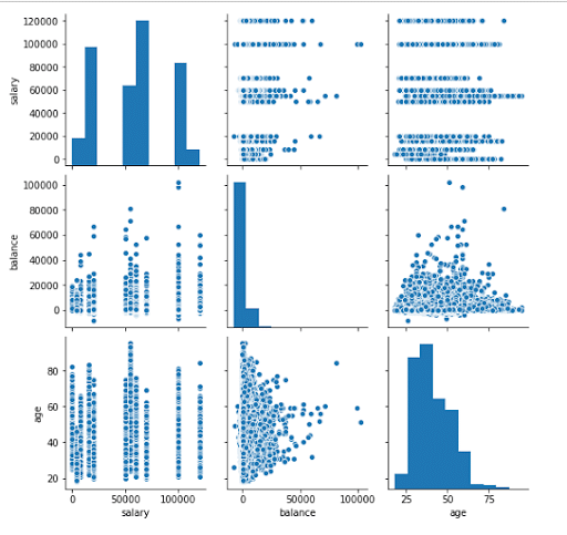
Figure 18: Pair diagrams of salary, balance and age

Correlation Matrix

A correlation matrix is ​​used to see the correlation between different variables. The correlation coefficient determines how two variables are correlated. The table below shows the correlation between salary, age and balance. Correlation tells you how one variable affects the other. This helps us determine how changes in one variable will also cause a change in the other.

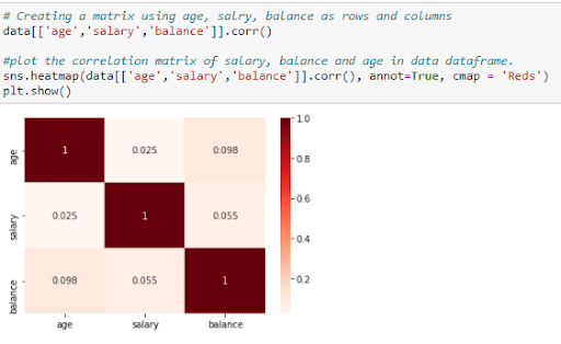
Figure 19: Correlation matrix between salary, balance and age

The above matrix tells us that balance, age and salary have a high correlation coefficient and influence each other. Age and salary have a lower correlation coefficient.

2. Numerical – Categorical Analysis

When one variable is of numeric type, and another is a categorical variable, you perform numeric-categorical analysis.

You can use the group by function to arrange the data into similar groups. Rows that have the same value in a particular column will be grouped. This way you can see the numerical occurrence of a certain category across a column. You can also group values ​​and find their average.

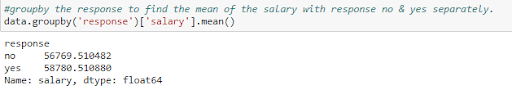
Figure 20: Grouping of response in relation to salary

The above values ​​tell you the average salary of the people who answered yes or no in the answer column.

You can also find the mean value of salary or the median value of the people who responded with yes and no in our survey.

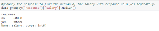
Figure 21: Median of group be of response regarding salary

You can also plot the box plot of response vs salary. A boxplot will show you the range of values ​​that fall under a certain category.

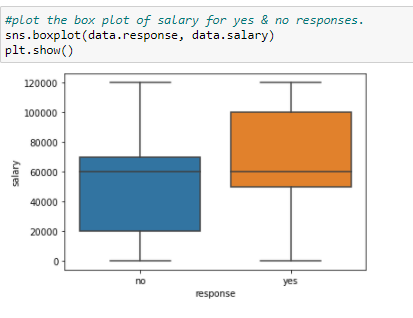
Figure 22: Boxplot of response in relation to salary

The above plot tells you that the salary range of people who said no to the survey is between 20k – 70k with a median salary of 60k, while the salary range of people who answered yes to the survey was between 50k – 100k with a median salary of 60K.

3. Categorical — Categorical Analysis

When both variables contain categorical data, you perform categorical-categorical analysis. First, convert the categorical response column into a numeric column with 1 corresponding to a positive response and 0 corresponding to a negative response.

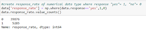
Figure 23: Changing from categorical to numerical values

Now compare the marital status of people with the response rate. The figure below tells you the average number of people who answered yes to the survey and their marital status.

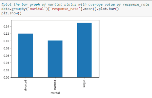
Figure 24: Changing from categorical to numerical values

Also, compare the average loan with the response rate.

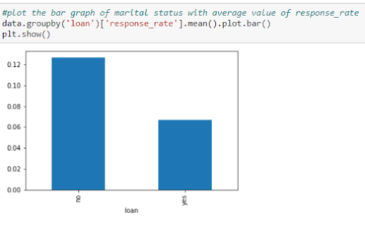
Figure 25: Changing from categorical to numerical values

You can conclude that people who have taken out a loan are likely to respond with a no to the survey.